The fundamental concept of differentiation in calculus is a powerful tool to help you understand the rate of change, and use it to solve problems. The chapter 3 in AP Calculus AB focuses primarily upon derivatives and applications. This comprehensive guide simplifies complex concepts to make them more accessible for all students. Let’s dig into the details.
Understanding Derivatives
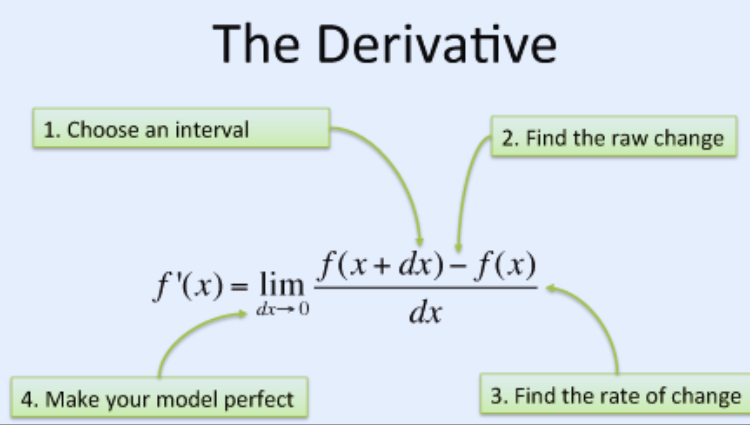
What Is a Derivative
A derivative is a measure of how a function alters as the input changes. It is the slope of a tangent to a curve. The derivative helps answer questions like:
- What is the speed of an object?
- What is the growth rate of a population?
Geometric Interpretation
Imagine a curve in a graph. The derivative at any point is the slope that “touches”, but does not cut through, the curve. The tangent is the line that crosses through it.
Differentiability & Continuity
A continuous function is required to create a derivative. A function is not differentiable where there are discontinuities, corners and cusps.
Also Check: Which Years Fit LS1 Intake Manifold on 5.3 Silverado?
Basic Rules for Differentiation
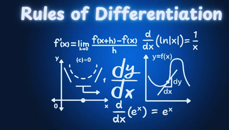
Power Rule
For any function f(x)=xnf(x) = x^n, the derivative is: ddx[xn]=nxn-1\fracddx[x^n] = n \cdot x^n-1
Product Rules
Use this formula to multiply two functions: (fg)=fg+fg(f cdotg)” = f’cdotg + fcdotg’
Quotient rule
For dividing two functions: (fg)’=f’g-fg’g2\left(\fracfg\right)’ = \fracf’ \cdot g – f \cdot g’g^2
Chain Rules
For composite functions f(g(x))f(g(x)): ddx[f(g(x))]=f'(g(x))g'(x)\fracddx[f(g(x))] = f'(g(x)) \cdot g'(x)
Applications and Derivatives
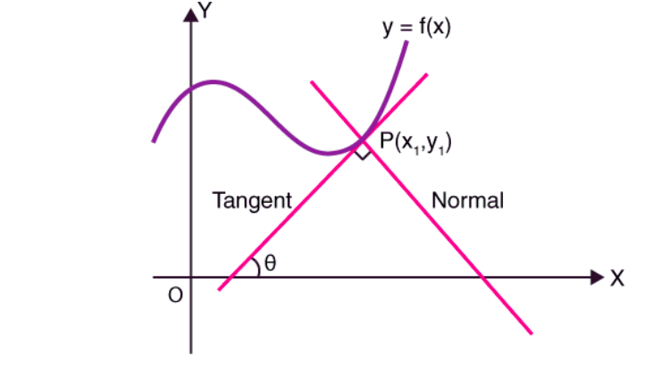
Find Tangent and Normal Lines
- Tangent line: Equation given by y=y_1=m(x-x1), where m=f(x1)m =f(x_1).
- Normal Line Perpendicular line: Its slope is (-1/m.
Acceleration and Velocity
- Velocity : Derived of position function s (t) s (t).
- Acceleration Second derivative of the velocity function s(t),s(t).
Related Rates
In these problems, you need to find the rate at which a quantity changes in relation with another. Use the chain rule in order to compare the derivatives.
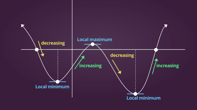
Extrema and Critical Points
Important Points
These critical points are found when f(x),f(x), or f(x),f(x), is not defined. These points can be candidates for saddle points, local minima or maxima.
Local Extrema
- Local extrema: Found by using the First Derivative Test
- Global extremes: Calculate the highest or lowest values of f(x).f(x).
Mean Value Theory (MVT)
Rolle’s Theorem
If a function (x)(x) is continuous, differentiable, and on [a,b][a and b], f (a)=f (b)f (a) = f (b), then there exists a c(a and b)c in (a and b) that has (f’ (c) = 0.
Mean Value Theory
For a differentiable function on [a,b][a, b]: f(b)-f(a)b-a=f'(c)\fracf(b) – f(a)b – a = f'(c)
The average rate of changes equals the instantaneous rates of change at a certain point.
Concavity & Inflection Points
Concavity
- A function is concave if f’ (x)>0f'(x) > 0.
- A function is concave downward when f’ (x)0f ” (x) 0.
Inflection points
Inflection points are the points where concavity changes. Inflection points are those where f(x), f(x), or f(x), f(x), is defined as 0, or f(x), f(x), or f(x), f(x), is undefined.
Curve Sketching
Combining the derivatives tools, we can:
- Critical points to consider
- Analyze the concavity of the surface and its inflection points.
- Find the asymptotes of behavior and its end.
- Draw a graph that accurately represents the function.
Advanced Application

Implicit Differentiation
Differentiate both sides in relation to xx and treat yy as (x.
Higher-Order Derivatives
The second derivative, f’ (x)f ‘(x), measures the rate of change f'(x)f ‘(x). Higher-order derivatives are used in physics, engineering and mathematics.
L’Hopital’s rule
For indeterminate forms like 0/00/0 or /: limx-cf(x)g(x)=limx-cf'(x)g'(x)\lim_x \to c \fracf(x)g(x) = \lim_x \to c \fracf'(x)g'(x)
Real-Life applications of derivatives
- Economics – Maximizing profits and minimising costs.
- Biology: Modeling population growth rates.
- Physics: Understanding Motion and Force
- Engineering: Designing Systems for Maximum Performance
Practice problems and solutions
**Example 1 : Find the derivative (f(x), = 3×2 + 5x + 2)
Solution:** ddx[3×2-5x+2]=6x-5\fracddx[3x^2 – 5x + 2] = 6x – 5
Example 2: An 10 ft ladder leans against the wall. How fast does the top slide down if the bottom is six feet from the wall and the bottom moves at 2 ft/s?
The Pythagorean formula and related rates are used to solve the problem.
Also Check: How the Delmag D-80 Hammer Boosts Construction Power
FAQs
What is the chain rule in calculus, and how is it applied in derivatives?
The chain rule is a fundamental concept in calculus used to differentiate composite functions. If you have a function f(g(x))f(g(x))f(g(x)), the chain rule states that the derivative of this composite function is the derivative of the outer function f′f’f′ evaluated at the inner function g(x)g(x)g(x), multiplied by the derivative of the inner function g′(x)g'(x)g′(x). In simpler terms:ddx[f(g(x))]=f′(g(x))⋅g′(x)\frac{d}{dx}[f(g(x))] = f'(g(x)) \cdot g'(x)dxd[f(g(x))]=f′(g(x))⋅g′(x)
This rule allows us to find derivatives of more complex functions by breaking them down into simpler parts.
How do implicit derivatives work in problems involving equations that aren’t explicitly solved for yyy?
Implicit differentiation is used when dealing with equations where yyy is not explicitly written as a function of xxx. Instead of solving for yyy, you differentiate both sides of the equation with respect to xxx, treating yyy as a function of xxx. When differentiating terms involving yyy, apply the chain rule (derivative of yyy is dydx\frac{dy}{dx}dxdy). After differentiating, solve for dydx\frac{dy}{dx}dxdy to find the slope of the curve at any point.
What are higher-order derivatives, and how are they calculated?
Higher-order derivatives are the derivatives of a function taken multiple times. The first derivative represents the rate of change of a function, the second derivative represents the rate of change of the first derivative (often related to concavity), and so on. To calculate higher-order derivatives, simply differentiate the function repeatedly. For example, the second derivative of a function f(x)f(x)f(x) is denoted as f′′(x)f”(x)f′′(x), and the third derivative is denoted as f′′′(x)f”'(x)f′′′(x). Each successive derivative provides more insight into the behavior of the function.
Conclusion
In conclusion, Chapter 3 of AB Calculus, titled Derivatives Simplified, provides a solid foundation for understanding the concept of derivatives, which are essential tools in calculus. By breaking down key principles such as the chain rule, implicit differentiation, and higher-order derivatives, this chapter equips students with the knowledge to tackle a wide range of problems involving rates of change and the behavior of functions.
Through practice and application, students can master these techniques and gain a deeper understanding of the mathematical underpinnings of real-world phenomena. Whether it’s optimizing functions, analyzing curves, or solving applied problems, the concepts learned in this chapter form the cornerstone of advanced calculus studies.